Range Control Chart

Build a control chart for subgroup ranges using either the conventional three-sigma approximation or exact probability limits from the distribution of the relative range $W = R / \sigma$.

Usage

cchart.R(x, n, type = c("norm", "tukey"), y = NULL)

Arguments

x: Phase II subgroup data accepted by qcc::qcc() for an "R" chart. Rows represent subgroups and columns observations within subgroups.
n: Integer subgroup size, at least 2. It is used to evaluate the actual false-alarm probability of the conventional chart and to obtain Tukey relative-range quantiles for the exact chart.
type: Either "norm" for the conventional three-sigma chart or "tukey" for exact equal-tail probability limits.
y: Phase I subgroup data used to estimate $\sigma$ through qcc::sd.R() when type = "tukey". It must be supplied for that method and have the same subgroup structure as x.

Value

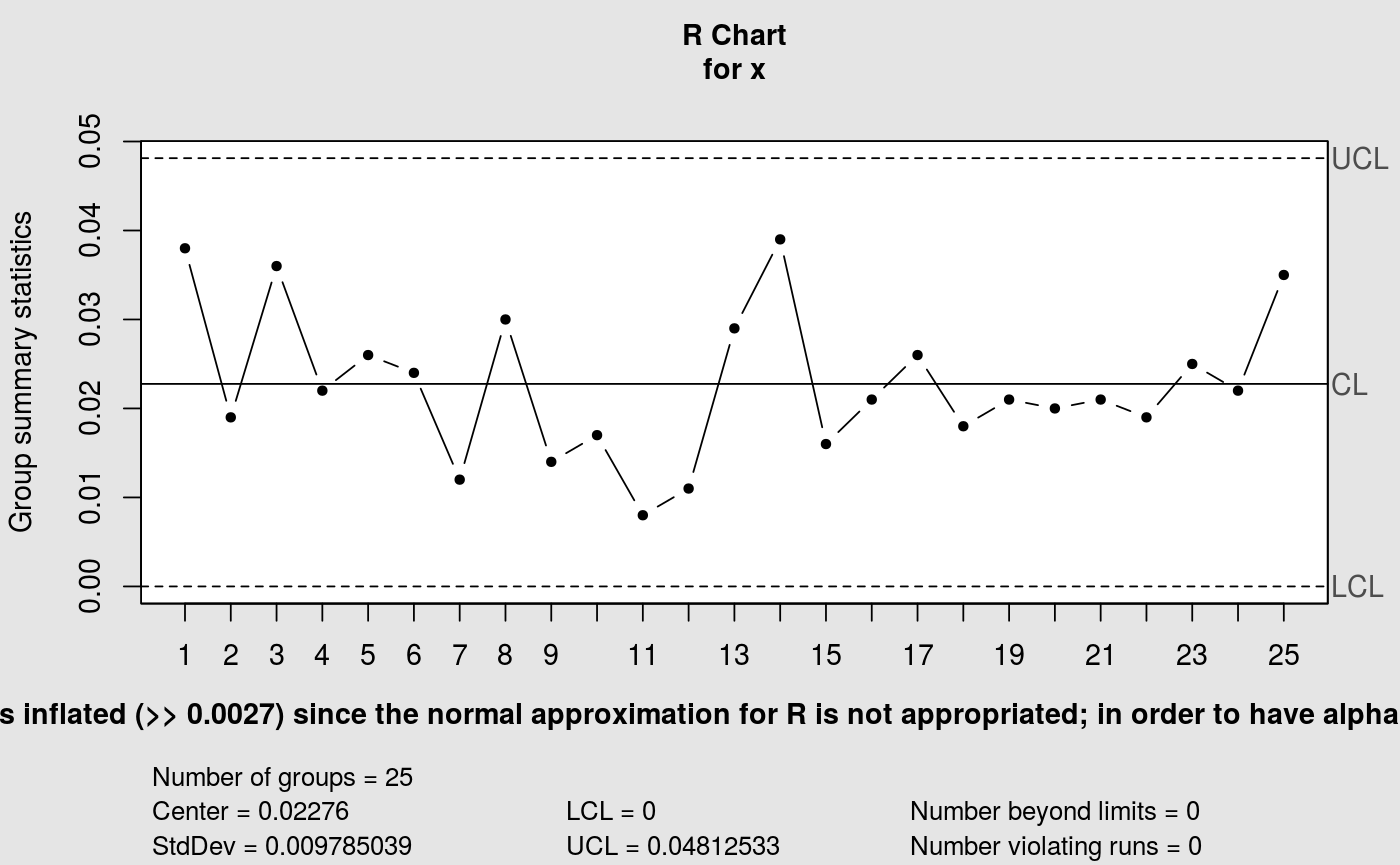
Invisibly, the "qcc" object returned by qcc::qcc(). The function also draws the chart. For type = "norm", a message is added below the plot showing the actual false-alarm probability returned by alpha.risk(n).

Details

The numerical limits are computed by r_shewhart_limits (for type = "norm") or r_exact_limits (for type = "tukey"), keeping the plotting wrapper separate from the pure limit calculations.

For type = "norm", limits are delegated to the standard qcc range-chart implementation. For type = "tukey", the lower and upper limits are $$\hat\sigma F_W^{-1}(0.00135;n)$$ and $$\hat\sigma F_W^{-1}(0.99865;n),$$ where $\hat\sigma$ is estimated from y and the quantiles are obtained with stats::qtukey().

Phase convention

The exact chart treats y as Phase I reference data and x as the plotted monitoring data. The conventional chart uses the standard estimation behavior of qcc::qcc() on x.

Errors

An error is raised for an unsupported type, for n < 2, or when y is omitted for the exact chart. Additional data validation is performed by qcc::qcc() and qcc::sd.R().

References

Barbosa, E. P., Gneri, M. A., and Meneguetti, A. (2013). Range control charts revisited: Simpler Tippett-like formulae, its practical implementation, and the study of false alarm. Communications in Statistics - Simulation and Computation, 42(2), 247–262. doi:10.1080/03610918.2011.639967 .

Author

Daniela R. Recchia, Emanuel P. Barbosa

Examples

data(pistonrings)
conventional <- cchart.R(pistonrings[1:25, ], 5)

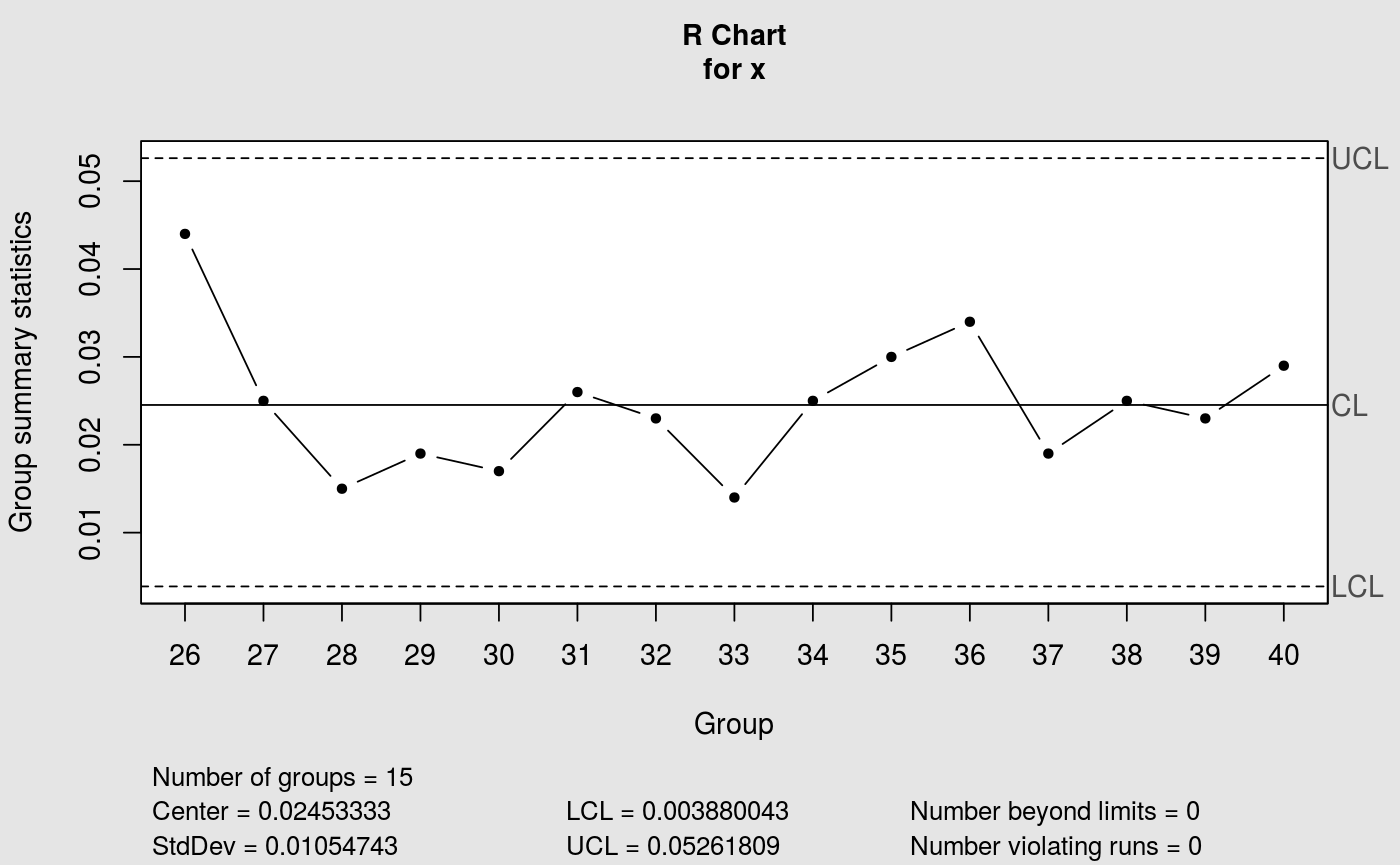
exact <- cchart.R(
    pistonrings[26:40, ], 5,
    type = "tukey",
    y = pistonrings[1:25, ]
)