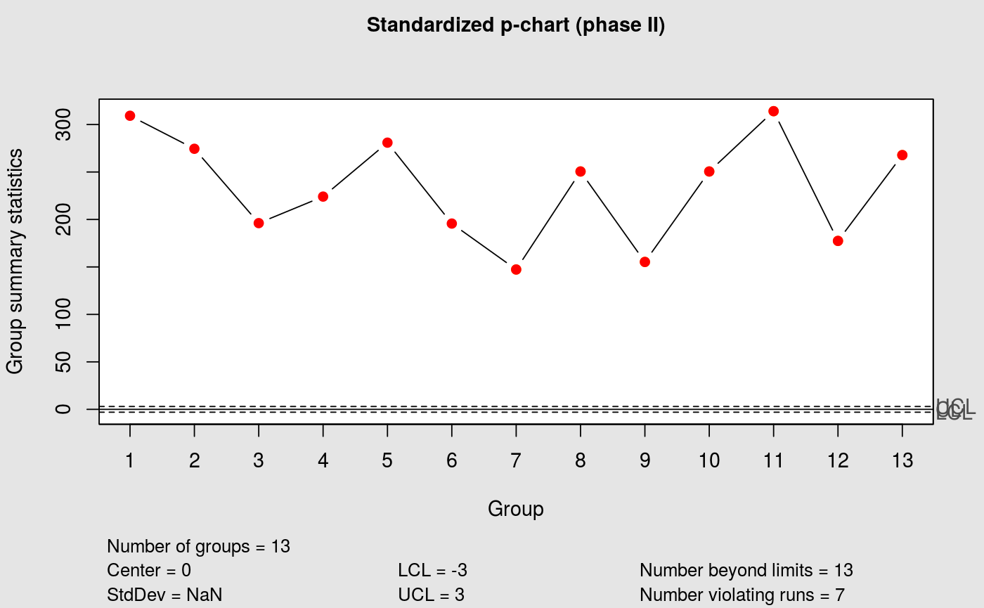
Build normal, Cornish-Fisher corrected, or standardized p charts.
Usage
cchart.p(
  x1 = NULL,
  n1 = NULL,
  type = "norm",
  p1 = NULL,
  x2 = NULL,
  n2 = NULL,
  phat = NULL,
  p2 = NULL,
  alpha = ALPHA
)
Arguments
- x1
Phase I nonconforming counts.
- n1
Phase I sample size or vector of sample sizes.
- type
Chart type. Accepted values are
"normal","cf1","cf2", and"standardized". The legacy aliases"norm","CF", and"std"remain supported;"CF"maps to"cf1".- p1
Phase I subgroup proportions. Used instead of
x1.- x2
Phase II nonconforming counts.
- n2
Phase II sample size or vector of sample sizes.
- phat
Known or previously estimated in-control proportion.
- p2
Phase II subgroup proportions. Used instead of
x2.- alpha
Nominal two-sided false alarm probability. Defaults to 0.0027.
Details
For a Phase I chart, n1 and exactly one of x1 or p1
must be supplied. For a Phase II chart, n2 and exactly one of
x2 or p2 must be supplied, together with Phase I information
or a known phat.
When sample sizes vary, the process proportion is estimated by the pooled
binomial estimator, \(sum(x_i) / sum(n_i)\), rather than by the unweighted
mean of subgroup proportions. The plotting wrapper uses two-sided limits;
use pchart_limits() directly for one-sided upper limits.
References
Montgomery, D. C. (2008). Introduction to Statistical Quality Control. Wiley.
Joekes, S. and Barbosa, E. P. (2013). An improved attribute control chart for monitoring non-conforming proportion in high quality processes. Control Engineering Practice, 21, 407–412. doi:10.1016/j.conengprac.2012.12.005 .
Examples
data(binomdata)
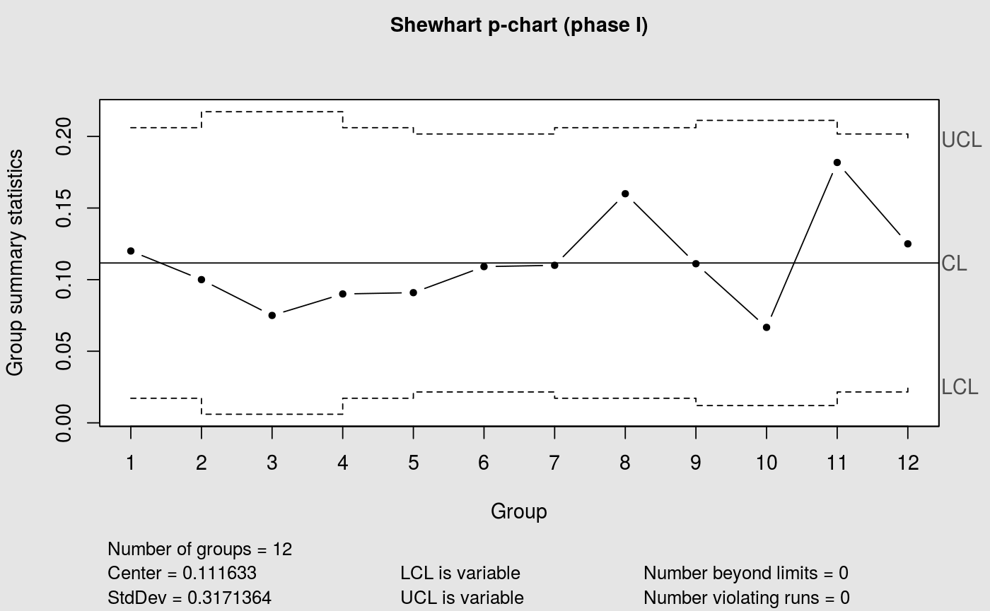
cchart.p(x1 = binomdata$Di[1:12], n1 = binomdata$ni[1:12])
 cchart.p(x1 = binomdata$Di[1:12], n1 = binomdata$ni[1:12],
type = "cf2", x2 = binomdata$Di[13:25],
n2 = binomdata$ni[13:25])
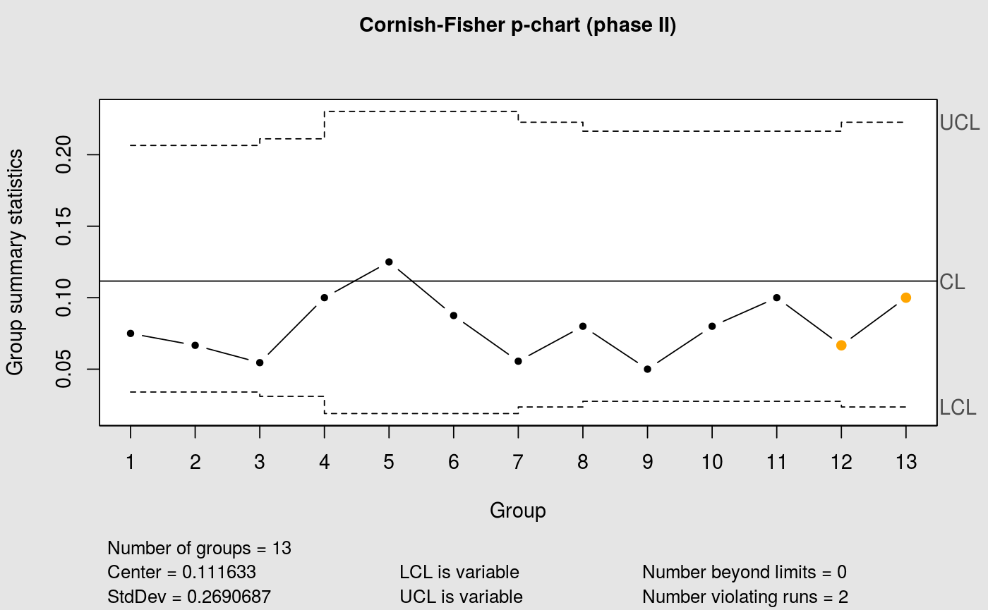
cchart.p(x1 = binomdata$Di[1:12], n1 = binomdata$ni[1:12],
type = "cf2", x2 = binomdata$Di[13:25],
n2 = binomdata$ni[13:25])
 cchart.p(type = "standardized", p2 = binomdata$Di[13:25] /
binomdata$ni[13:25], n2 = binomdata$ni[13:25],
phat = 0.1115833)
cchart.p(type = "standardized", p2 = binomdata$Di[13:25] /
binomdata$ni[13:25], n2 = binomdata$ni[13:25],
phat = 0.1115833)