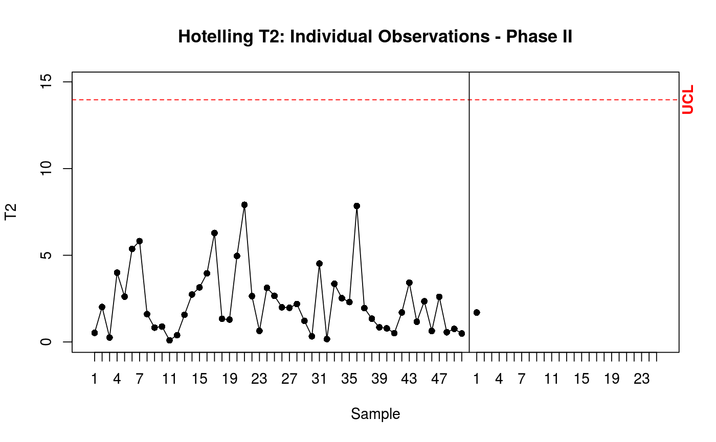
Build or update a Phase II T² chart. Can optionally display Phase I reference data. Limits: For \(n = 1\): \(UCL = (p(m+1)(m-1))/(m^2-mp) \times qf(1-\alpha, p, m-p)\). For \(n > 1\): \(UCL = (p(m+1)(n-1))/(mn-m-p+1) \times qf(1-\alpha, p, mn-m-p+1)\).
Arguments
- T2II
Vector with Phase II T² values (from
T2.2).- m
Number of Phase I subgroups.
- n
Subgroup size.
- j
Index of the current Phase II sample (1-based).
- t
Maximum x-axis limit (number of Phase II samples to show).
- p
Number of variables.
- datum
Optional. Phase I data array to display reference points.
- stats
Optional. Phase I statistics to compute T² if not provided.
- T2
Optional. Pre-computed Phase I T² values.
Phase convention
Phase II monitoring. The vertical dashed line separates Phase I (left) from Phase II (right).
References
Montgomery, D.C., (2009). "Introduction to Statistical Quality Control". Chapter 11. Wiley.
Examples
mu <- c(5.682, 88.22)
Sigma <- miscTools::symMatrix(c(3.770, -5.495, 13.53), 2)
datum <- data.1(20, 10, mu, Sigma)
estat <- stats(datum, 20, 10, 2)
datum2 <- data.2(estat, 10, p = 2)
T2II <- T2.2(datum2, estat, 10)
# For the first sample j = 1. T2II is a vector with the value of the first T2 statistic.
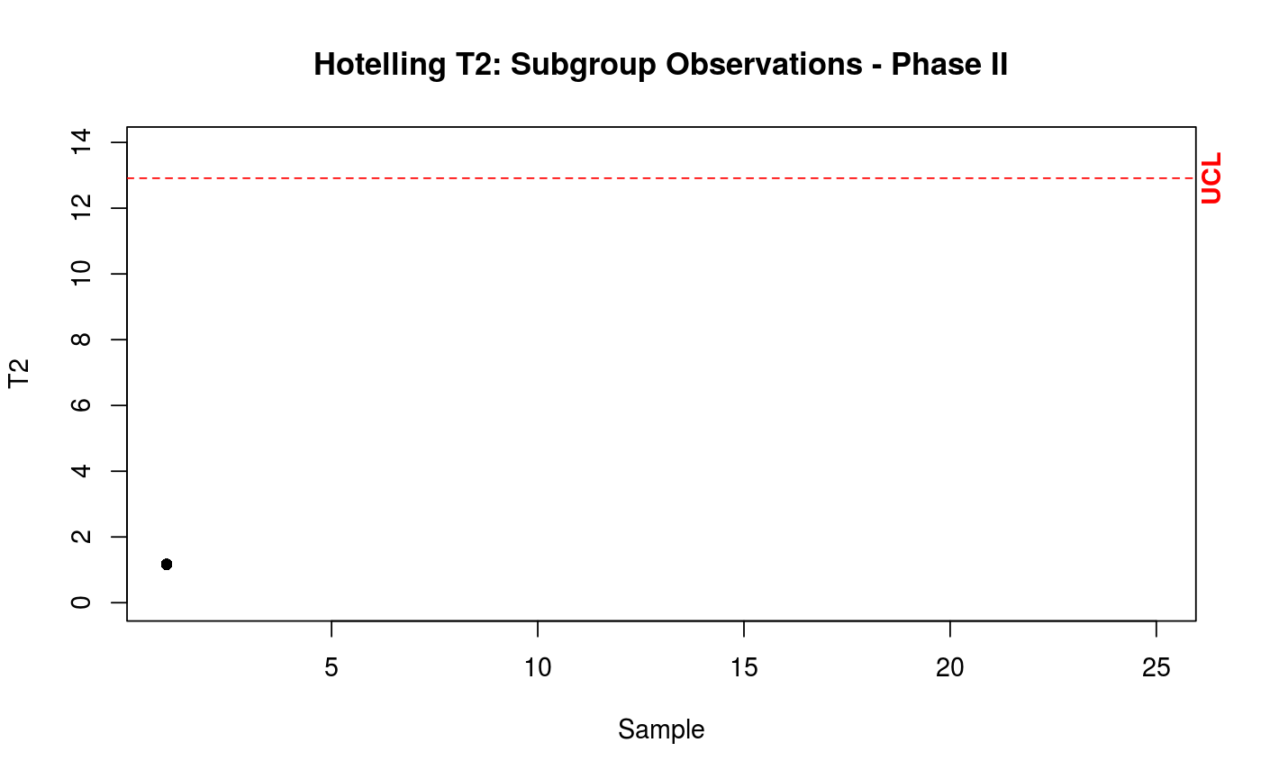
cchart.T2.2(T2II, 20, 10, 1, 25, 2)
 # Same of the above, but now showing the phase I data set.
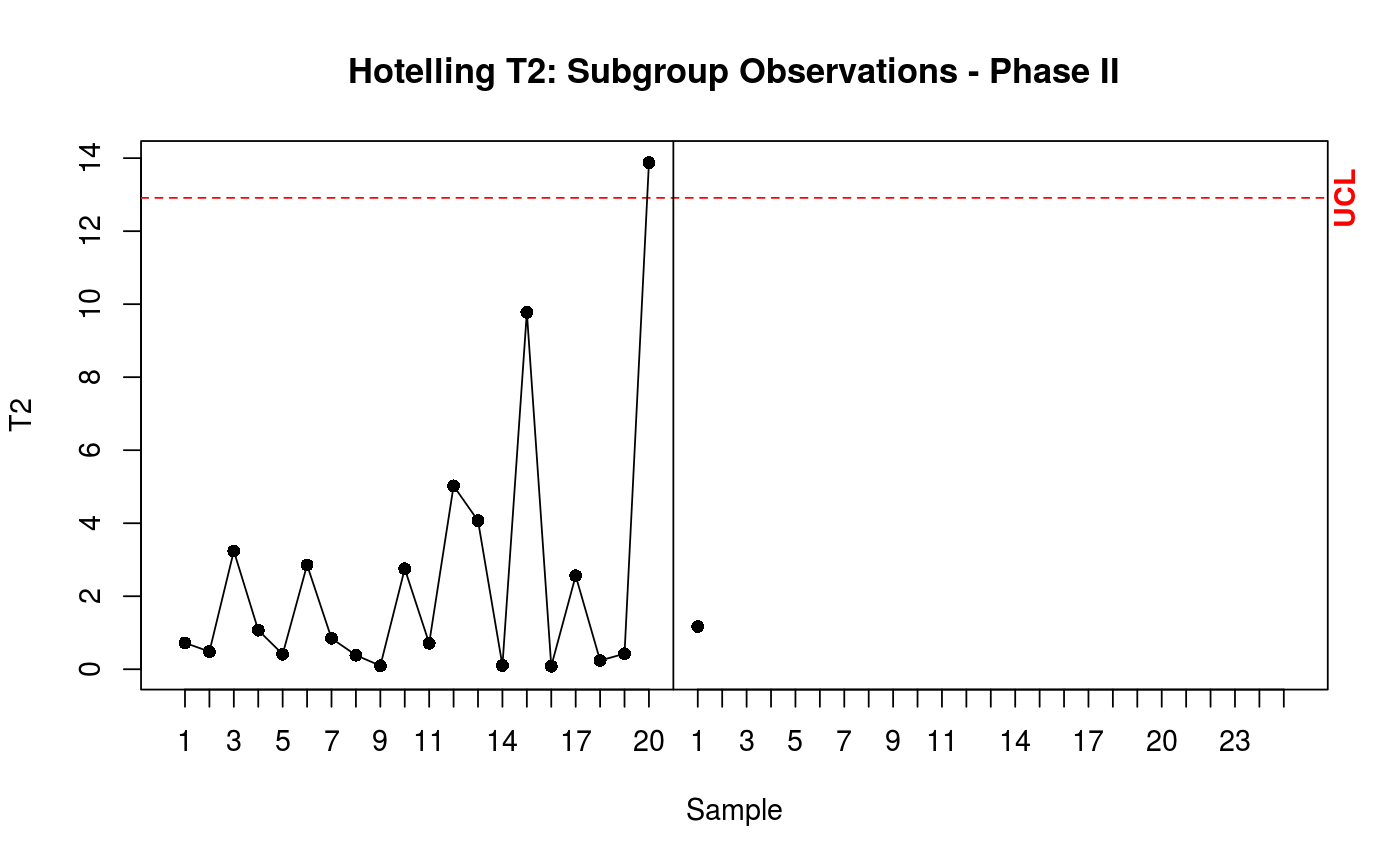
cchart.T2.2(T2II, 20, 10, 1, 25, 2, datum = datum)
# Same of the above, but now showing the phase I data set.
cchart.T2.2(T2II, 20, 10, 1, 25, 2, datum = datum)
 #Example with individual observations
datum <- data.1(50, 1, mu, Sigma)
estat <- stats(datum, 50, 1, 2)
datum2 <- data.2(estat, 1, p = 2)
T2II <- T2.2(datum2, estat, 1)
# For the first sample j = 1. T2II is a vector with the value of the first T2 statistic.
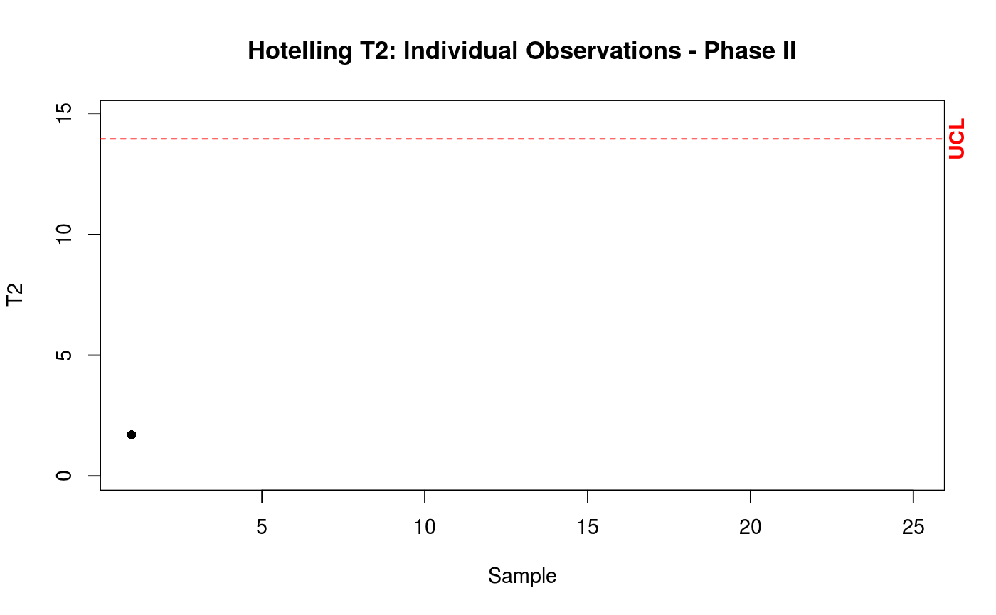
cchart.T2.2(T2II, 50, 1, 1, 25, 2)
#Example with individual observations
datum <- data.1(50, 1, mu, Sigma)
estat <- stats(datum, 50, 1, 2)
datum2 <- data.2(estat, 1, p = 2)
T2II <- T2.2(datum2, estat, 1)
# For the first sample j = 1. T2II is a vector with the value of the first T2 statistic.
cchart.T2.2(T2II, 50, 1, 1, 25, 2)
 # Same of the above, but now showing the phase I data set.
cchart.T2.2(T2II, 50, 1, 1, 25, 2, datum = datum)
# Same of the above, but now showing the phase I data set.
cchart.T2.2(T2II, 50, 1, 1, 25, 2, datum = datum)