When to use IQCC: exact and corrected control charts • IQCC

Purpose

IQCC implements Improved Quality Control Charts: control charts with exact, corrected, standardized, or simulation-based limits for situations where classical Shewhart-type approximations may be poorly calibrated.

The package is not intended to replace general-purpose statistical process control packages. Instead, it is useful when the monitoring statistic is bounded, discrete, skewed, strongly non-normal, or based on small samples. In those settings, the usual three-sigma limits can produce a false-alarm probability that differs meaningfully from the nominal value.

Positioning in the R ecosystem

IQCC is a specialized package for exact and corrected control-chart limits, especially for small samples, rare nonconformities, asymmetric statistics, and selected multivariate monitoring problems.

Use a general SPC package when the goal is a broad control-chart workflow. Use IQCC when the main concern is whether classical limits are statistically well calibrated for the distribution and sample size at hand.

Current implemented methods

The current package includes:

cchart.R() and cchart.S() for range and standard-deviation charts;
pchart_limits(), pchart_alpha_risk(), and cchart.p();
uchart_limits(), uchart_alpha_risk(), and cchart.u();
the DS-np design and monitoring family;
Hotelling T-squared Phase I and Phase II functions;
generalized-variance limits, risk diagnostics, and charts;
auxiliary tr(V) trace-statistic limits, risk diagnostics, and charts.

Executed example: corrected p-chart limits

The chunk below is evaluated when the vignette and the pkgdown site are built. It prints the limits and their exact binomial false-alarm probability.

data(binomdata)

p0 <- sum(binomdata$Di[1:12]) / sum(binomdata$ni[1:12])
lim_p <- pchart_limits(p = p0, n = 20, type = "cf2")
risk_p <- pchart_alpha_risk(
  p = p0,
  n = 20,
  lcl = lim_p$lcl,
  ucl = lim_p$ucl
)

data.frame(
  p0 = p0,
  lcl = lim_p$lcl,
  center = lim_p$center,
  ucl = lim_p$ucl,
  actual_alpha = risk_p,
  arl0 = ifelse(risk_p == 0, Inf, 1 / risk_p)
)
#>          p0 lcl    center       ucl actual_alpha     arl0
#> 1 0.1134454   0 0.1134454 0.3653831 0.0009758464 1024.751

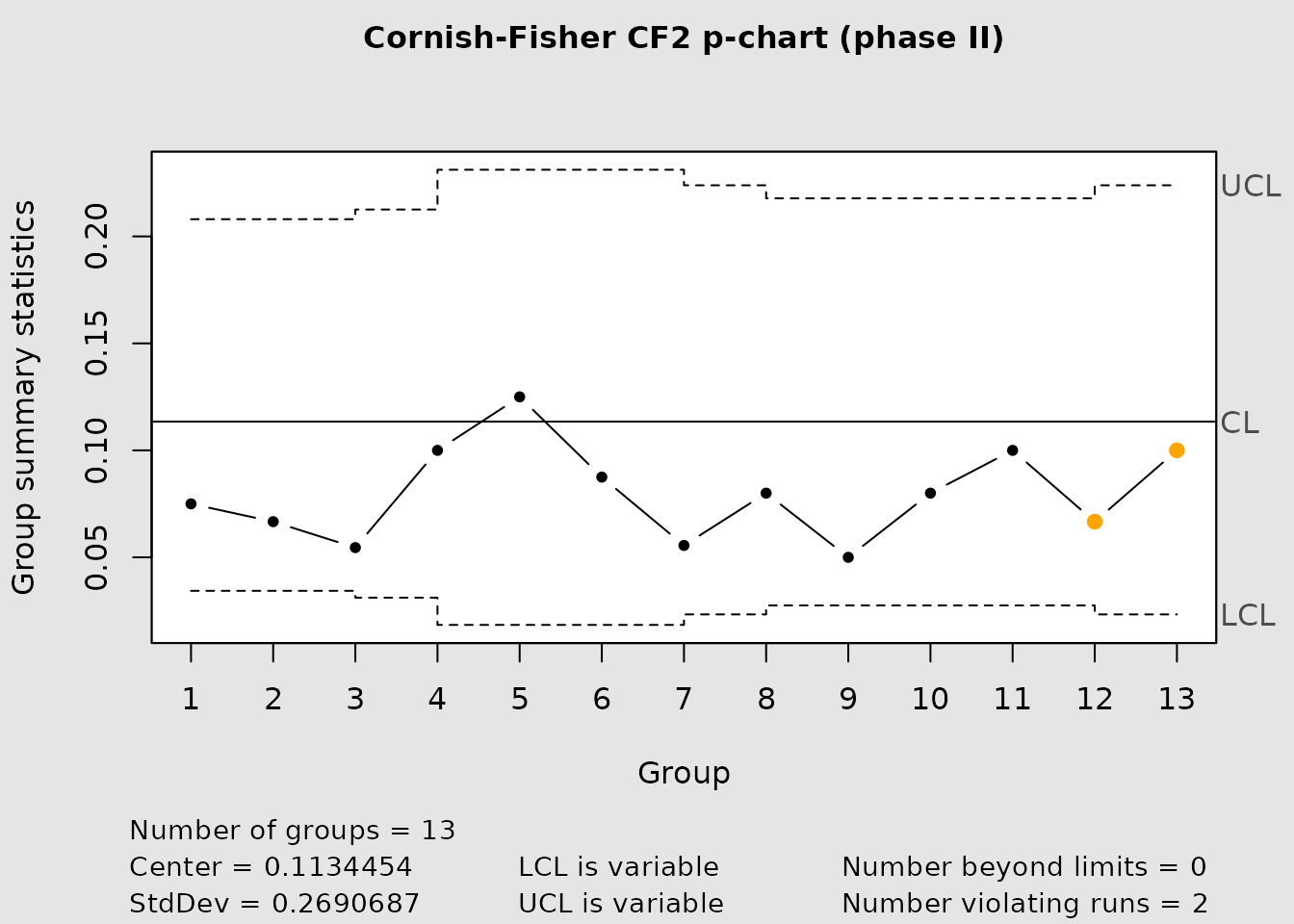
The operational chart itself is also executed and produces a figure in the published article.

cchart.p(
  x1 = binomdata$Di[1:12],
  n1 = binomdata$ni[1:12],
  type = "cf2",
  x2 = binomdata$Di[13:25],
  n2 = binomdata$ni[13:25]
)

Executed example: DS-np operating characteristics

The published small-sample design can be evaluated directly without an expensive search.

n1 <- 34
n2 <- 162
wl <- 1.5
ucl1 <- 2.5
ucl2 <- 4.5
p0 <- 0.005
p1 <- 0.0075

perf_dsnp <- data.frame(
  quantity = c("ARL0", "ARL1", "ASS0"),
  value = c(
    dsnp_arl(p0, n1, n2, wl, ucl1, ucl2)$arl,
    dsnp_arl(p1, n1, n2, wl, ucl1, ucl2)$arl,
    dsnp_ass(p0, n1, n2, wl, ucl1)$ass
  )
)
perf_dsnp
#>   quantity     value
#> 1     ARL0 803.41143
#> 2     ARL1 193.22286
#> 3     ASS0  35.93534

A compact search is used in the vignette so that CI remains fast while still executing the design algorithm.

small_search <- dsnp_limits(
  p0 = 0.05,
  n1 = 5,
  n2 = 10,
  alpha = 0.05,
  p1 = 0.10,
  max_results = 5
)
small_search$best[, c("wl", "ucl1", "ucl2", "arl0", "arl1", "ass0")]
#>    wl ucl1 ucl2     arl0     arl1     ass0
#> 1 0.5  1.5  2.5 24.91743 5.951221 7.036266

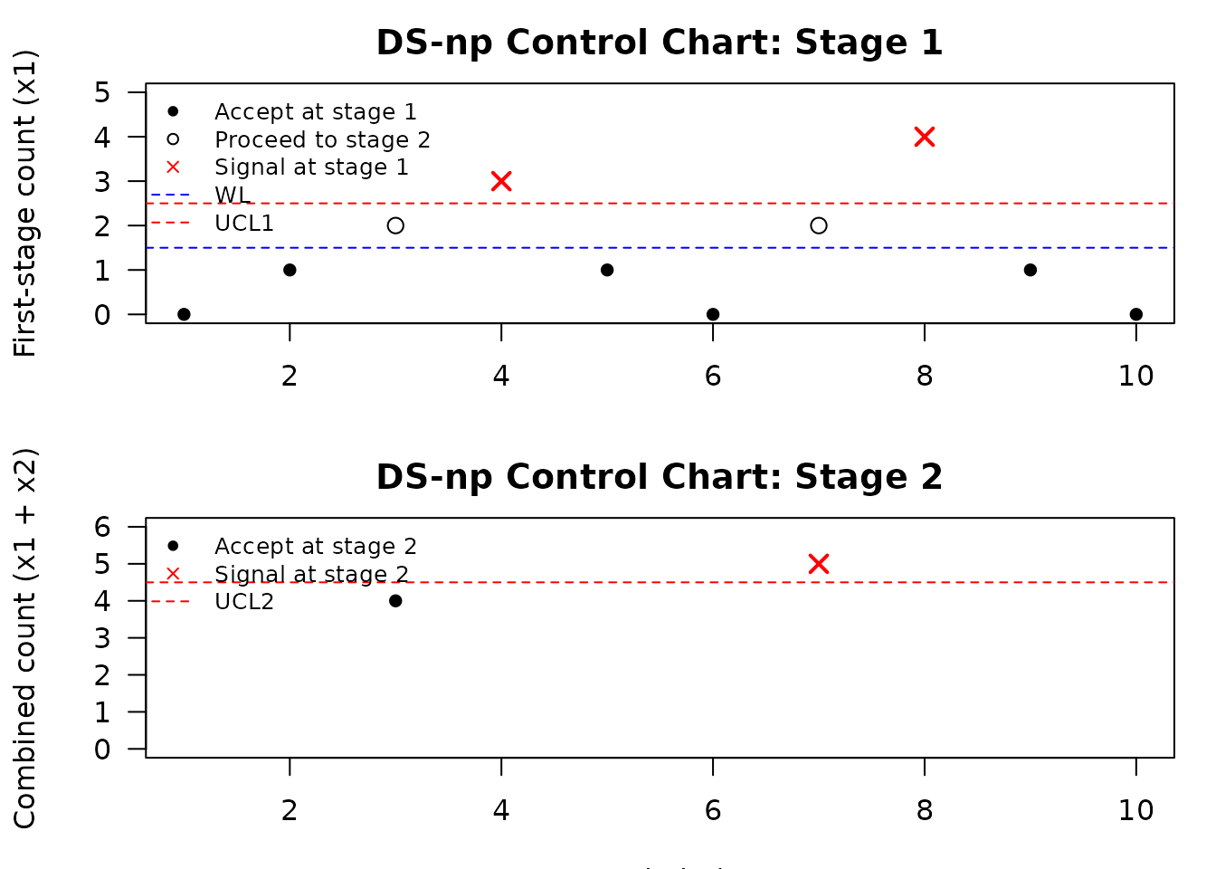
The chart is built with explicit limits, which makes the displayed decision rule reproducible.

x1 <- c(0, 1, 2, 3, 1, 0, 2, 4, 1, 0)
x2 <- c(NA, NA, 2, NA, NA, NA, 3, NA, NA, NA)

chart_dsnp <- cchart.DSnp(
  x1,
  n1 = 10,
  n2 = 20,
  p0 = 0.05,
  x2 = x2,
  wl = 1.5,
  ucl1 = 2.5,
  ucl2 = 4.5,
  plot = TRUE
)

chart_dsnp$performance
#> $arl0
#> [1] 58.35236
#> 
#> $ass0
#> [1] 11.4927
#> 
#> $p_signal0
#> [1] 0.01713727

Executed example: generalized variance

gv_comparison <- do.call(
  rbind,
  lapply(c("normal", "cf", "exact"), function(method) {
    limits <- gv_limits(
      n = 10,
      p = 2,
      det_sigma = 0.5320,
      type = method
    )
    data.frame(method = method, lcl = limits$lcl,
               center = limits$center, ucl = limits$ucl)
  })
)
gv_comparison
#>   method lcl    center      ucl
#> 1 normal   0 0.4728889 1.428685
#> 2     cf   0 0.4728889 2.160305
#> 3  exact   0 0.4728889 2.153629

set.seed(123)
gv_data <- array(rnorm(8 * 8 * 2), dim = c(8, 8, 2))
cchart.GV(
  gv_data,
  Sigma = diag(2),
  type = "exact",
  plot = TRUE
)

#> Generalized Variance Control Chart
#>   Dimension: p = 2 ; subgroup size n = 8 
#>   Subgroups: 8 (Phase I: 8 ; Phase II: 0 )
#>   Limits: exact / upper ; nominal alpha = 0.0027 
#>   Covariance: supplied Sigma 
#>   LCL = 0 ; center = 0.8571 ; UCL = 4.622 
#>   Signals: 0

cat("<!-- IQCC_EXECUTED_POSITIONING -->\n")

Development principles

Numerical calculations should remain separated from plotting functions, new methods should be validated against published examples whenever possible, and IQCC should remain complementary to the broader R statistical process-control ecosystem.