Getting started with IQCC

What IQCC is for

IQCC provides improved quality-control charts for settings in which familiar normal, three-sigma limits can be poorly calibrated. These settings include small subgroups, rare nonconformities, discrete or skewed statistics, and multivariate variability. The package emphasizes exact limits where they are available, distributional corrections where they are justified, and explicit calculation of the actual false-alarm risk.

IQCC complements qcc. The latter provides a broad statistical process-control framework, and IQCC reuses it for several plots. IQCC adds specialized numerical functions and plotting wrappers for corrected attribute charts, double-sampling plans, exact range limits, generalized variance, and the auxiliary trace statistic. Use qcc for a general SPC workflow; use IQCC when the calibration of a particular small-sample or non-normal statistic matters.

Numerical functions and chart wrappers

The preferred workflow is to calculate and inspect a design before drawing a chart. For example, pchart_limits() returns the limits without plotting, and pchart_alpha_risk() evaluates their exact binomial false-alarm probability. The wrapper cchart.p() applies the selected method to observed subgroups and returns the underlying qcc object invisibly.

p_limits <- pchart_limits(p = 0.015, n = 20, type = "cf2")
p_risk <- pchart_alpha_risk(
  p = 0.015,
  n = 20,
  lcl = p_limits$lcl,
  ucl = p_limits$ucl
)

data.frame(
  lcl = p_limits$lcl,
  center = p_limits$center,
  ucl = p_limits$ucl,
  actual_alpha = p_risk
)
#>   lcl center       ucl actual_alpha
#> 1   0  0.015 0.1303192  0.003178083

The same separation is available for p and u limits, DS-np operating characteristics, generalized variance, and tr(V). The older R, S, and Hotelling interfaces remain primarily chart-oriented; their plotting functions should not be mistaken for generic numerical limit APIs.

Phase I, Phase II, and reference parameters

Phase I data establish or assess the in-control reference. Phase II data are new subgroups monitored against limits fixed from that reference. IQCC uses method-specific argument names:

Chart	Phase I	Phase II	Known reference
p	x1 or p1	x2 or p2	phat
u	x1 or u1	x2 or u2	lambda
R	y for exact limits	x	none in the wrapper
Hotelling T-squared	data.1(), stats(), T2.1()	data.2(), T2.2()	Phase I estimates
generalized variance	x1	x2	Sigma
tr(V)	x	newdata	Sigma0

When phat, lambda, Sigma, or Sigma0 is supplied, it is treated as an external in-control reference. Otherwise, the relevant wrapper estimates it from Phase I. Plug-in limits based on estimated parameters do not automatically account for the additional estimation uncertainty.

Input formats

Attribute charts accept one-dimensional vectors. Counts are paired with their sample or inspection sizes; proportions and rates can be supplied directly.

p_counts <- c(0, 1, 0, 2, 1, 0)
p_sizes <- c(40, 50, 45, 60, 55, 50)
p_proportions <- p_counts / p_sizes

u_counts <- c(1, 0, 3, 2, 1, 4)
u_sizes <- c(10, 12, 15, 11, 14, 13)
u_rates <- u_counts / u_sizes

data.frame(
  p_count = p_counts,
  p_proportion = p_proportions,
  u_count = u_counts,
  u_rate = u_rates
)
#>   p_count p_proportion u_count     u_rate
#> 1       0   0.00000000       1 0.10000000
#> 2       1   0.02000000       0 0.00000000
#> 3       0   0.00000000       3 0.20000000
#> 4       2   0.03333333       2 0.18181818
#> 5       1   0.01818182       1 0.07142857
#> 6       0   0.00000000       4 0.30769231

Multivariate variability functions accept a list of subgroup matrices, a subgroup-by-observation-by-variable array, or a matrix made by stacking equal subgroups. Here all three representations contain the same data.

g1 <- cbind(
  x = c(-1, 0, 1, -1, 1),
  y = c(-1, 1, 0, 1, -1)
)
g2 <- sweep(g1, 2, c(0.2, -0.1), "+")
g3 <- g1 %*% matrix(c(1.1, 0.1, 0, 0.9), nrow = 2)
groups <- list(g1, g2, g3)

group_array <- array(NA_real_, dim = c(3, 5, 2))
for(i in seq_along(groups))
  group_array[i, , ] <- groups[[i]]

stacked_groups <- do.call(rbind, groups)

cbind(
  from_list = gv_stat(groups),
  from_array = gv_stat(group_array),
  from_stacked_matrix = gv_stat(stacked_groups, size = 5)
)
#>      from_list from_array from_stacked_matrix
#> [1,] 0.9375000  0.9375000           0.9375000
#> [2,] 0.9375000  0.9375000           0.9375000
#> [3,] 0.9188438  0.9188438           0.9188438

The legacy Hotelling helpers use a different array convention: observation-by-variable-by-subgroup. Check dim() before passing an array between the two families.

Corrected p and u charts

The numerical p and u functions support normal, first-order Cornish-Fisher ("cf1"), and second-order Cornish-Fisher ("cf2") limits. Their chart wrappers additionally support standardized observations.

p_methods <- do.call(
  rbind,
  lapply(c("normal", "cf1", "cf2"), function(method) {
    lim <- pchart_limits(0.02, n = 40, type = method)
    data.frame(method = method, lcl = lim$lcl, ucl = lim$ucl,
               applicable = lim$applicable)
  })
)

u_methods <- do.call(
  rbind,
  lapply(c("normal", "cf1", "cf2"), function(method) {
    lim <- uchart_limits(0.20, n = 10, type = method)
    data.frame(method = method, lcl = lim$lcl, ucl = lim$ucl)
  })
)

p_methods
#>   method lcl        ucl applicable
#> 1 normal   0 0.08640732      FALSE
#> 2    cf1   0 0.11840677       TRUE
#> 3    cf2   0 0.10890324       TRUE
u_methods
#>   method lcl       ucl
#> 1 normal   0 0.6242608
#> 2    cf1   0 0.7575918
#> 3    cf2   0 0.7340222

The p-chart workflow below estimates the in-control proportion from Phase I, computes the Phase II limits explicitly, and then constructs the Phase II chart. This makes the sequence from reference data to monitoring data visible.

p_phase1_counts <- c(1, 0, 1, 2, 0, 1, 1, 0)
p_phase1_sizes <- rep(50, length(p_phase1_counts))
p_phase1_estimate <- sum(p_phase1_counts) / sum(p_phase1_sizes)
p_phase2_limits <- pchart_limits(
  p = p_phase1_estimate,
  n = p_sizes,
  type = "cf2"
)

p_chart <- cchart.p(
  type = "cf2",
  x1 = p_phase1_counts,
  n1 = p_phase1_sizes,
  x2 = p_counts,
  n2 = p_sizes
)
c(
  estimated_phat = p_phase1_estimate,
  smallest_phase2_ucl = min(p_phase2_limits$ucl),
  largest_phase2_ucl = max(p_phase2_limits$ucl)
)
#>      estimated_phat smallest_phase2_ucl  largest_phase2_ucl 
#>          0.01500000          0.07768796          0.09407003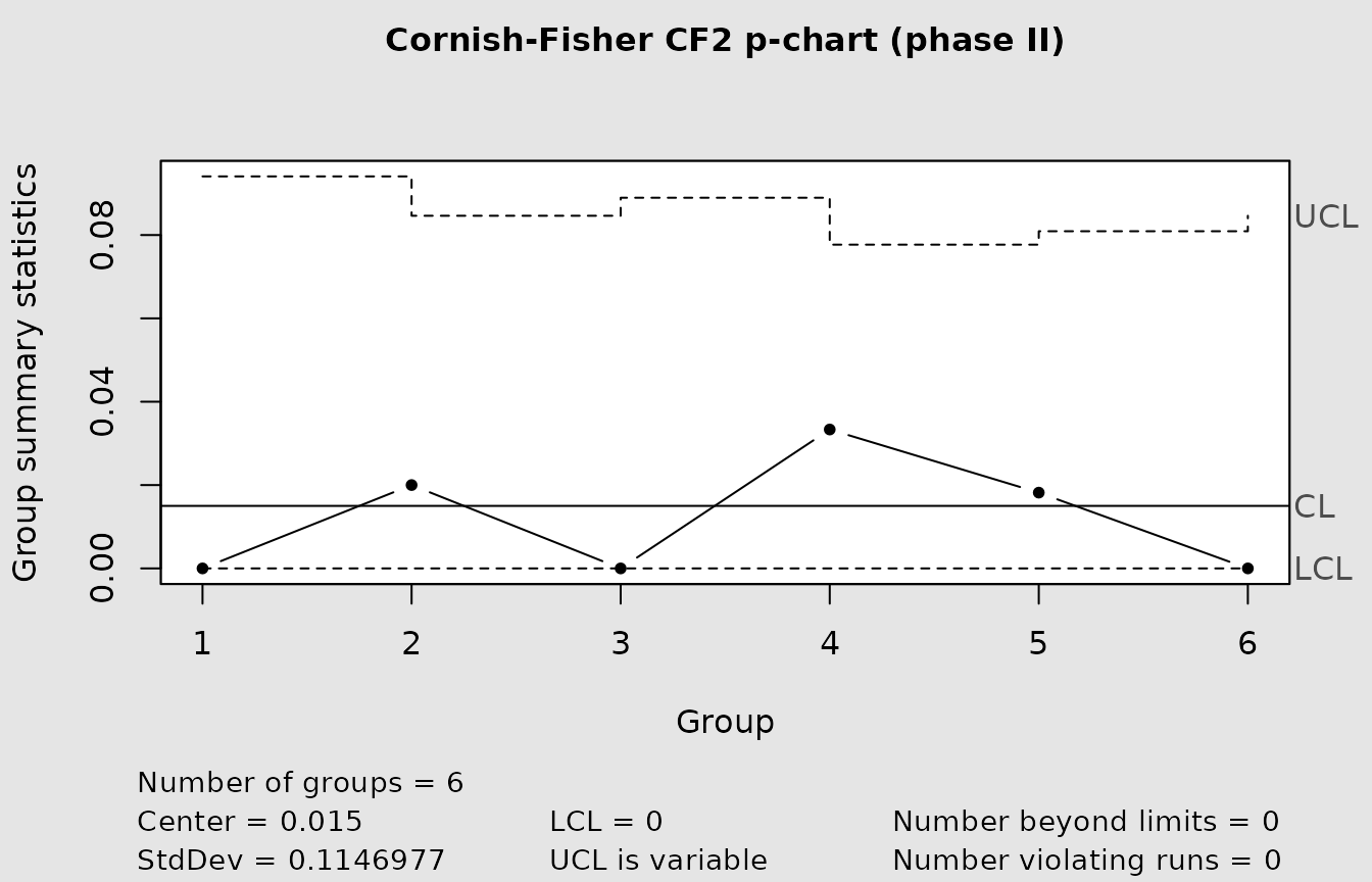

The u chart uses a known rate and direct rate input to demonstrate the prospective alternative.

u_chart <- cchart.u(
  type = "standardized",
  u2 = u_rates,
  n2 = u_sizes,
  lambda = 0.15
)
class(u_chart)
#> [1] "qcc"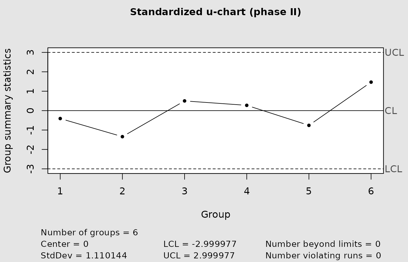

For estimated parameters, supply Phase I counts or proportions/rates instead. With unequal sizes, IQCC uses pooled estimators: sum(counts) / sum(sizes).

Double-sampling np

A DS-np plan can accept or signal after the first sample, or inspect a second sample when the first count falls in the warning region. The pure functions calculate acceptance probability, ARL, and ASS for explicit limits.

ds_plan <- list(
  p0 = 0.005,
  p1 = 0.010,
  n1 = 50,
  n2 = 242,
  wl = 1.5,
  ucl1 = 2.5,
  ucl2 = 4.5
)

data.frame(
  arl0 = with(ds_plan, dsnp_arl(p0, n1, n2, wl, ucl1, ucl2)$arl),
  arl1 = with(ds_plan, dsnp_arl(p1, n1, n2, wl, ucl1, ucl2)$arl),
  ass0 = with(ds_plan, dsnp_ass(p0, n1, n2, wl, ucl1)$ass)
)
#>       arl0     arl1     ass0
#> 1 200.0416 21.37162 55.82639

The chart object records every stage decision as well as its design and operating characteristics.

ds_chart <- cchart.DSnp(
  x1 = c(0, 1, 2, 3, 1),
  x2 = c(NA, NA, 2, NA, NA),
  n1 = 10,
  n2 = 20,
  p0 = 0.05,
  p1 = 0.10,
  wl = 1.5,
  ucl1 = 2.5,
  ucl2 = 4.5,
  plot = FALSE
)
ds_chart$data
#>   index x1 x2 total         stage signal
#> 1     1  0 NA    NA  accept_first  FALSE
#> 2     2  1 NA    NA  accept_first  FALSE
#> 3     3  2  2     4 accept_second  FALSE
#> 4     4  3 NA    NA  signal_first   TRUE
#> 5     5  1 NA    NA  accept_first  FALSE
ds_chart$performance
#> $arl0
#> [1] 58.35236
#> 
#> $ass0
#> [1] 11.4927
#> 
#> $p_signal0
#> [1] 0.01713727
#> 
#> $arl1
#> [1] 7.531628
#> 
#> $ass1
#> [1] 13.8742
#> 
#> $p_signal1
#> [1] 0.1327734

dsnp_limits() searches limits for fixed n1 and n2; dsnp_design() searches across supplied sample-size ranges. These are exhaustive discrete searches over the requested ranges, not continuous optimization routines.

Range and standard-deviation charts

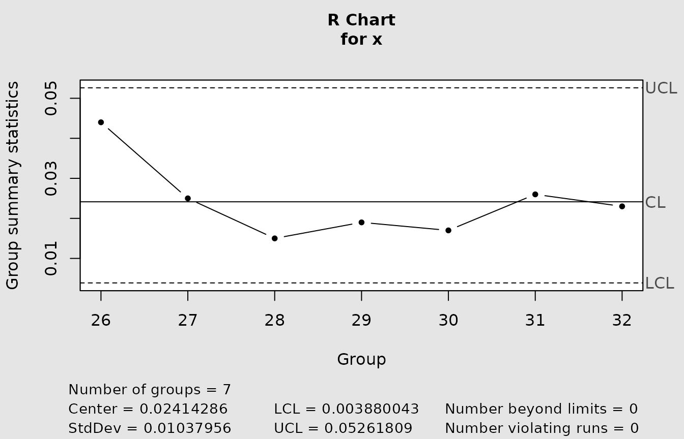
Rows are subgroups and columns are observations for the R and S wrappers. The range chart offers conventional ("norm") and exact relative-range ("tukey") limits. The S chart offers normalized ("n") and exact chi-square ("e") limits.

data(pistonrings)
r_chart <- cchart.R(
  x = pistonrings[26:32, ],
  n = 5,
  type = "tukey",
  y = pistonrings[1:25, ]
)

class(r_chart)
#> [1] "qcc"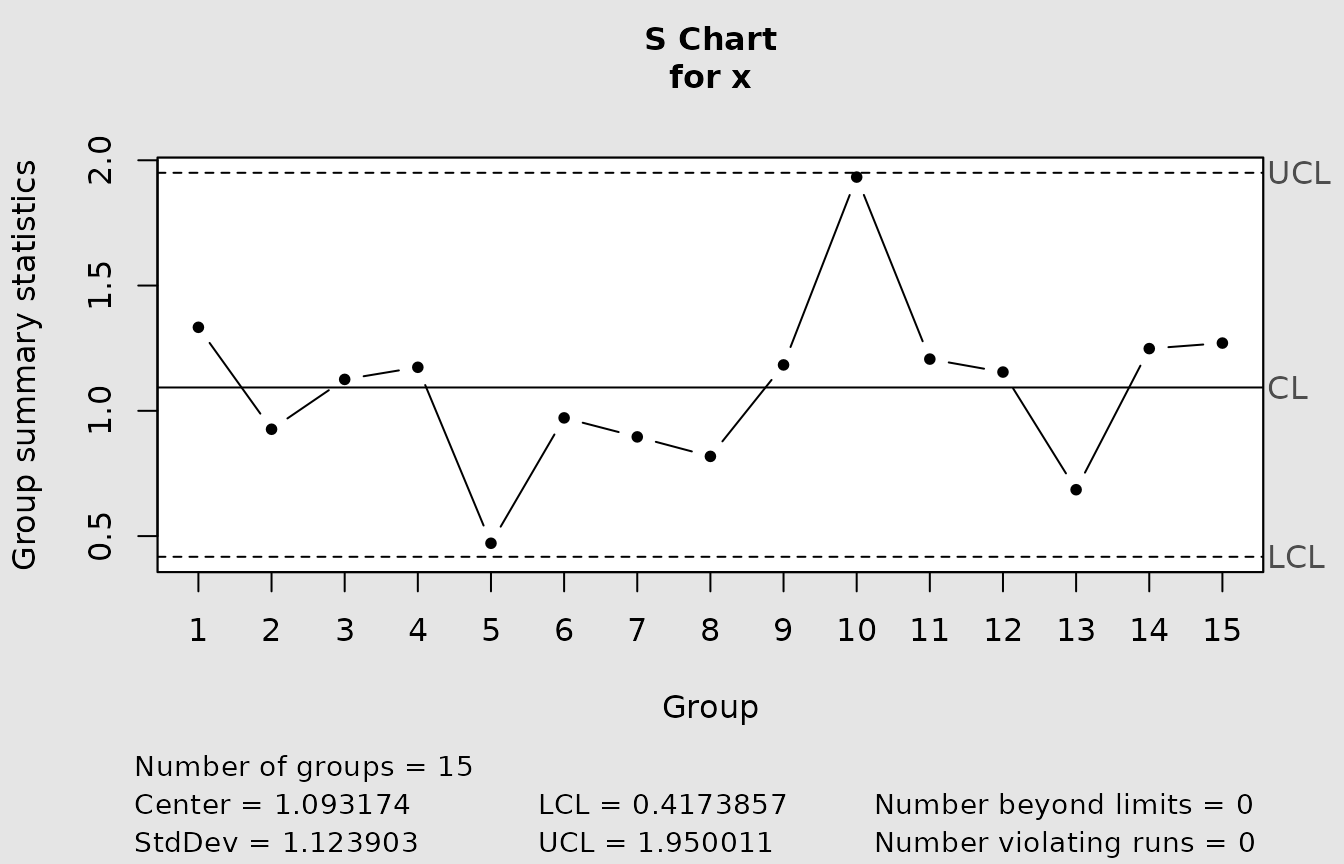

data(softdrink)
s_chart <- cchart.S(softdrink, type = "e", m = 10)

class(s_chart)
#> [1] "qcc"

Use alpha.risk(n) to inspect the actual risk of the conventional R chart, and table.qtukey() to inspect relative-range quantiles. The current R and S wrappers do not expose a complete pure numerical limits object analogous to pchart_limits().

Hotelling T-squared

The Hotelling workflow estimates the Phase I mean and covariance, computes a T-squared statistic for each subgroup, and evaluates later subgroups against the Phase II design. Its simulation helpers return arrays in observation-by-variable-by-subgroup order.

set.seed(2026)
hotelling_phase1 <- data.1(
  m = 8,
  n = 5,
  mu = c(0, 0),
  Sigma = diag(2)
)
hotelling_reference <- IQCC::stats(hotelling_phase1, m = 8, n = 5, p = 2)
hotelling_t2_phase1 <- T2.1(hotelling_reference, m = 8, n = 5)

hotelling_phase2 <- data.2(hotelling_reference, n = 5, p = 2)
hotelling_t2_phase2 <- T2.2(
  hotelling_phase2,
  hotelling_reference,
  n = 5
)

cchart.T2.1(hotelling_t2_phase1, m = 8, n = 5, p = 2)
c(phase1_max = max(hotelling_t2_phase1), phase2 = hotelling_t2_phase2)
#> phase1_max     phase2 
#>   8.114591   3.856580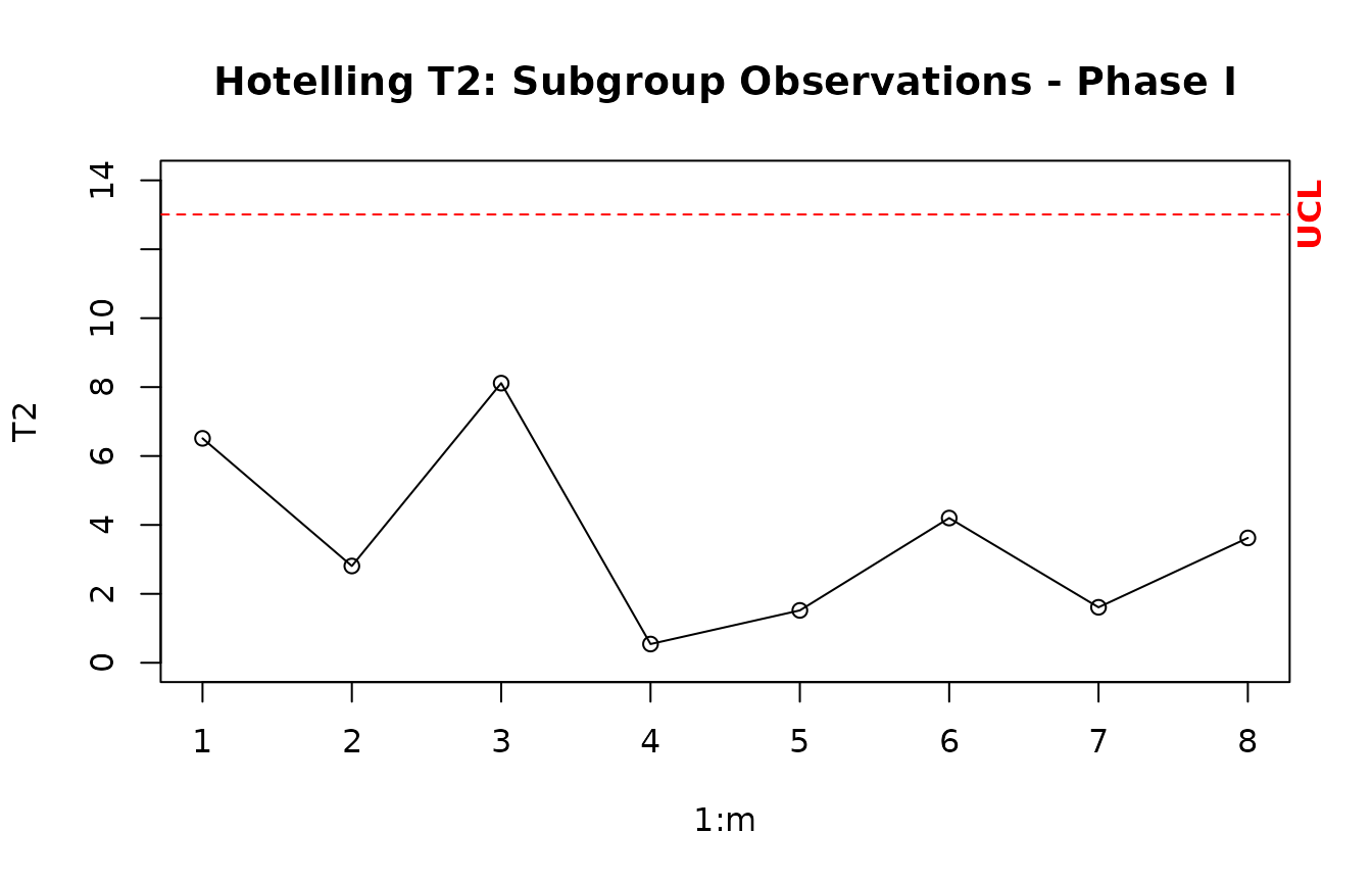

cchart.T2.2() draws the operational Phase II chart. The Phase I and Phase II limits differ, so the two plotting functions are not interchangeable.

Generalized variance and tr(V)

For each multivariate subgroup, gv_stat() computes the determinant of the sample covariance matrix. trv_stat() computes (n - 1) tr(Sigma0^-1 S). The determinant and standardized trace detect different covariance changes and are complementary.

data.frame(
  subgroup = seq_along(groups),
  generalized_variance = gv_stat(groups),
  trace_statistic = trv_stat(groups, Sigma0 = diag(2))
)
#>   subgroup generalized_variance trace_statistic
#> 1        1            0.9375000             8.0
#> 2        2            0.9375000             8.0
#> 3        3            0.9188438             7.9

Dimension-two generalized-variance limits have an exact implementation. Normal, Cornish-Fisher, and simulation methods are also available. Simulation is reproducible when seed is supplied.

gv_method_table <- do.call(
  rbind,
  lapply(c("normal", "cf", "exact"), function(method) {
    lim <- gv_limits(n = 5, p = 2, det_sigma = 1, type = method)
    data.frame(method = method, center = lim$center, ucl = lim$ucl)
  })
)
gv_simulated <- gv_limits(
  n = 5,
  p = 2,
  det_sigma = 1,
  type = "simulation",
  nsim = 2000,
  seed = 2026
)

gv_method_table
#>   method center      ucl
#> 1 normal   0.75 3.305568
#> 2     cf   0.75 6.769365
#> 3  exact   0.75 6.288749
gv_simulated[c("type", "ucl", "nsim", "seed")]
#> $type
#> [1] "simulation"
#> 
#> $ucl
#> [1] 5.379544
#> 
#> $nsim
#> [1] 2000
#> 
#> $seed
#> [1] 2026

The trace statistic has an exact chi-square upper limit under a known in-control covariance matrix. Its simulation option is mainly a diagnostic comparison with that same null distribution.

gv_chart <- cchart.GV(
  x1 = groups[1:2],
  x2 = groups[3],
  type = "cf",
  plot = FALSE
)

trv_chart <- cchart.trV(
  x = groups[1:2],
  newdata = groups[3],
  Sigma0 = diag(2),
  type = "chisq",
  plot = FALSE
)

summary(gv_chart)
#> Generalized Variance Control Chart
#>   Dimension: p = 2 ; subgroup size n = 5 
#>   Subgroups: 3 (Phase I: 2 ; Phase II: 1 )
#>   Limits: cf / upper ; nominal alpha = 0.0027 
#>   Covariance: estimated from Phase I subgroups 
#>   LCL = 0 ; center = 0.8036 ; UCL = 7.253 
#>   Signals: 0
summary(trv_chart)
#> Trace-Statistic Control Chart
#>   Dimension: p = 2 ; subgroup size n = 5 
#>   Subgroups: 3 (Phase I: 2 ; Phase II: 1 )
#>   Limits: chisq ; nominal alpha = 0.0027 ; df = 8 
#>   Covariance: supplied Sigma0 
#>   Center = 8 ; UCL = 23.57 
#>   Signals: 0

If Sigma or Sigma0 is omitted, Phase I covariance information is used as a plug-in estimate. Phase II observations never update that reference. The nominal known-parameter distribution does not include the extra uncertainty introduced by estimating the reference from a finite Phase I sample.

Choosing a method

• normal uses conventional or moment-matched Gaussian limits.
• cf1 and cf2 are first- and second-order Cornish-Fisher methods for p and u charts. Generalized variance uses type = "cf" with cf_order = 1 or 2.
• exact refers to a supported distributional result, not to simulation. Its scope depends on the statistic and dimension.
• standardized is available in the p and u plotting wrappers and places subgroup observations on a z scale.
• simulation uses Monte Carlo quantiles. Set nsim and seed, and report simulation error when using the result scientifically.
• The exact tr(V) method is named "chisq", reflecting its chi-square null distribution.

An exact known-parameter limit can become a plug-in operational limit when its reference parameter is estimated. Report that distinction explicitly.

Inspecting limits and signals

Modern IQCC chart objects are lists. Inspect their components rather than reading values from a plot.

data.frame(
  chart = c("DS-np", "generalized variance", "tr(V)"),
  n_statistics = c(
    nrow(ds_chart$data),
    length(gv_chart$statistics),
    length(trv_chart$statistics)
  ),
  n_signals = c(
    sum(ds_chart$data$signal),
    length(gv_chart$out.of.control),
    length(trv_chart$out.of.control)
  )
)
#>                  chart n_statistics n_signals
#> 1                DS-np            5         1
#> 2 generalized variance            3         0
#> 3                tr(V)            3         0

gv_chart$limits[c("lcl", "center", "ucl", "type", "alpha")]
#> $lcl
#> [1] 0
#> 
#> $center
#> [1] 0.8035714
#> 
#> $ucl
#> [1] 7.252891
#> 
#> $type
#> [1] "cf"
#> 
#> $alpha
#> [1] 0.0027

For p and u charts, inspect the returned qcc object, including its statistics, limits, and violations components. For DS-np, |S|, and tr(V), summary() provides a compact account of parameters, phases, limits, and signals.

IQCC generally signals strict excursions beyond a limit. For generalized variance, a point signals when it is below the LCL or above the UCL; equality does not signal. The tr(V) chart signals only when the statistic is strictly above its UCL. DS-np uses integer thresholds derived from its fractional limits, so inspect ds_chart$limits before interpreting a boundary count.

Common errors

• Do not supply both counts and proportions/rates for the same attribute-chart phase.
• Match every count vector with a sample-size vector of the same length, unless a scalar size is intentionally recycled.
• Do not use p1 to mean the same thing everywhere: in cchart.p() it is a vector of Phase I proportions, while in DS-np functions it is the scalar out-of-control process proportion.
• For DS-np, provide a second-stage count whenever the first-stage count lies in the warning zone; use NA only when the second sample is not required.
• For multivariate variability, use subgroup-by-observation-by-variable arrays; the legacy Hotelling helpers use observation-by-variable-by-subgroup arrays.
• Generalized variance requires more observations than variables in every subgroup. Sigma and Sigma0 must be symmetric positive-definite matrices with the correct dimension.
• Do not describe a simulated limit as exact, and do not assume a plug-in limit has known-parameter coverage.

Further documentation

Read vignette("high-quality-processes", package = "IQCC") for corrected p charts and DS-np plans, vignette("statistical-foundations", package = "IQCC") for formulas and published validations, and vignette("iqcc-positioning", package = "IQCC") for the package’s scope. Function manuals contain the complete input validation, return values, decision inequalities, and method-specific limitations.